Rincón de Práctica Stata#
Datos Panel usando Stata#
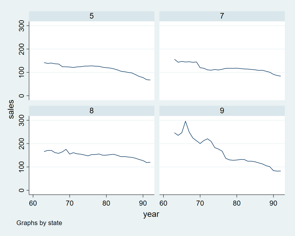
Data#
import pandas as pd
import ipystata
%%stata
import delimited http://www-eio.upc.edu/~pau/cms/rdata/csv/Ecdat/Cigar.csv, clear
xtset state year
(encoding automatically selected: ISO-8859-1)
(10 vars, 1,380 obs)

Panel variable: state (strongly balanced)
 Time variable: year, 63 to 92
         Delta: 1 unit
%%stata
  xtline sales if state>4&state<10
Modelo FE#
\[sales_{it}=\alpha_i+x'_{it}\beta+u_{it}\]
con \(\alpha_i\) efecto fijo asociado al estado.
%%stata
  xtreg sales price pop pop16 ndi, fe r
Fixed-effects (within) regression               Number of obs     =      1,380
Group variable: state                           Number of groups  =         46

R-squared:                                      Obs per group:
     Within  = 0.2844                                         min =         30
     Between = 0.2740                                         avg =       30.0
     Overall = 0.1558                                         max =         30

                                                F(4,45)           =      32.69
corr(u_i, Xb) = 0.1106                          Prob > F          =     0.0000

                                 (Std. err. adjusted for 46 clusters in state)
------------------------------------------------------------------------------
             |               Robust
       sales | Coefficient  std. err.      t    P>|t|     [95% conf. interval]
-------------+----------------------------------------------------------------
       price |  -.3513145   .1682916    -2.09   0.043    -.6902711   -.0123579
         pop |  -.0087096   .0059391    -1.47   0.149    -.0206716    .0032523
       pop16 |   .0112986   .0092271     1.22   0.227    -.0072858    .0298831
         ndi |   .0010731   .0020565     0.52   0.604    -.0030689    .0052152
       _cons |   141.4895   6.238091    22.68   0.000     128.9253    154.0536
-------------+----------------------------------------------------------------
     sigma_u |  24.842588
     sigma_e |  14.898338
         rho |  .73548253   (fraction of variance due to u_i)
------------------------------------------------------------------------------
Modelo RE#
%%stata
  xtreg sales price pop pop16 ndi, re r
Random-effects GLS regression                   Number of obs     =      1,380
Group variable: state                           Number of groups  =         46

R-squared:                                      Obs per group:
     Within  = 0.2842                                         min =         30
     Between = 0.2384                                         avg =       30.0
     Overall = 0.1624                                         max =         30

                                                Wald chi2(4)      =     123.33
corr(u_i, X) = 0 (assumed)                      Prob > chi2       =     0.0000

                                 (Std. err. adjusted for 46 clusters in state)
------------------------------------------------------------------------------
             |               Robust
       sales | Coefficient  std. err.      z    P>|z|     [95% conf. interval]
-------------+----------------------------------------------------------------
       price |  -.3676653   .1650456    -2.23   0.026    -.6911487   -.0441818
         pop |  -.0087648   .0069247    -1.27   0.206     -.022337    .0048073
       pop16 |   .0111637   .0099851     1.12   0.264    -.0084067    .0307342
         ndi |   .0012399   .0020123     0.62   0.538    -.0027041    .0051839
       _cons |   142.0622   7.412126    19.17   0.000     127.5347    156.5897
-------------+----------------------------------------------------------------
     sigma_u |  21.045538
     sigma_e |  14.898338
         rho |  .66616216   (fraction of variance due to u_i)
------------------------------------------------------------------------------
Modelo Two-way FE#
\[sales_{it}=\mu_i+\mu_t+x'_{it}\beta+u_{it}\]
con \(\alpha_i\) efecto fijo asociado al estado y \(\mu_t\) efecto fijo asociado al año.
%%stata
  reghdfe sales price pop pop16 ndi, absorb(state year) vce(r)
(MWFE estimator converged in 2 iterations)

HDFE Linear regression                            Number of obs   =      1,380
Absorbing 2 HDFE groups                           F(   4,   1301) =      47.62
                                                  Prob > F        =     0.0000
                                                  R-squared       =     0.8467
                                                  Adj R-squared   =     0.8375
                                                  Within R-sq.    =     0.2304
                                                  Root MSE        =    12.4910

------------------------------------------------------------------------------
             |               Robust
       sales | Coefficient  std. err.      t    P>|t|     [95% conf. interval]
-------------+----------------------------------------------------------------
       price |  -.8296836   .0894201    -9.28   0.000    -1.005107   -.6542602
         pop |  -.0025949   .0019491    -1.33   0.183    -.0064187    .0012288
       pop16 |   .0040946   .0025701     1.59   0.111    -.0009475    .0091366
         ndi |  -.0057015   .0008145    -7.00   0.000    -.0072994   -.0041037
       _cons |    221.843   7.428401    29.86   0.000     207.2701     236.416
------------------------------------------------------------------------------

Absorbed degrees of freedom:
-----------------------------------------------------+
 Absorbed FE | Categories  - Redundant  = Num. Coefs |
-------------+---------------------------------------|
       state |        46           0          46     |
        year |        30           1          29     |
-----------------------------------------------------+
Panel Dinámico#
\[sales_{i,t}=sales_{i,t-1}+\mu_i+x'_{i,t}\beta+u_{i,t}\]
con \(\alpha_i\) efecto fijo asociado al estado
%%stata
  xtabond sales price pop pop16 ndi, vce(robust)
Arellano–Bond dynamic panel-data estimation     Number of obs     =      1,288
Group variable: state                           Number of groups  =         46
Time variable: year
                                                Obs per group:
                                                              min =         28
                                                              avg =         28
                                                              max =         28

Number of instruments =    411                  Wald chi2(5)      =   15775.72
                                                Prob > chi2       =     0.0000
One-step results
                                  (Std. err. adjusted for clustering on state)
------------------------------------------------------------------------------
             |               Robust
       sales | Coefficient  std. err.      z    P>|z|     [95% conf. interval]
-------------+----------------------------------------------------------------
       sales |
         L1. |   .8646417   .0236058    36.63   0.000     .8183752    .9109082
             |
       price |  -.0661191   .0353343    -1.87   0.061    -.1353731    .0031348
         pop |  -.0046988   .0030159    -1.56   0.119    -.0106099    .0012122
       pop16 |   .0056149   .0036481     1.54   0.124    -.0015352     .012765
         ndi |  -.0000592   .0003699    -0.16   0.873    -.0007841    .0006658
       _cons |   23.41488   3.986634     5.87   0.000     15.60122    31.22854
------------------------------------------------------------------------------
Instruments for differenced equation
        GMM-type: L(2/.).sales
        Standard: D.price D.pop D.pop16 D.ndi
Instruments for level equation
        Standard: _cons